
One of the often touted examples of the power of quantum computers is their ability to run Shor’s Algorithm, which is a way to quickly find the prime factors of a number, and hence defeat many of the encryption schemes used today.
There are many good explanations of how Shor’s algorithm works, like this more conceptual overview, this more mathematical explainer, or this article which not only explains the algorithm, but also the fundamentals of how a quantum computer operates. I’m not going to re-explain the algorithm, but instead I’m going to walk through an example, and hopefully give some insight into what the q-bits are doing.
The code in this post is written in Julia, and using the Gadfly package for visualizations.
If you want to play along, you can install Julia, or you can head over to tmpnb and create a new Julia notebook (I wrote this while using version 0.3.2). If you’ve installed Julia on your own, make sure you install Gadfly using
Pkg.add("Gadfly")
Then make sure you’re using Gadly in your session with
using Gadfly
And now we’re ready to walk through Shor’s algorithm.
We start by picking what number to factor. For speed and simplicity I’m going to choose $m=21 = 7 * 3$. We pick a number $r$, and we will find the order of $r$ in the modular group of $m$, which is 21 for us. I’m going to pick $r=2$, but any number that isn’t already a factor of $m$ will work. (And if you’ve picked a factor of $m$ congratulations, you just factored your number!). Setting these variable in Julia (I will be using >> to show the results of these commands).
m = 7*3
r = 2
m,r, gcd(m,r)
>> 21,2,1
Next we need to prepare our set of qubits. Just how many we need depends on a couple of things, how large our number $m$ is, and how accurate we want our answer to be. We will have a pair of registers, whose sizes we need to decide on.
We are going to calculate $r^a \mod m$ for many values of a, and the first register will contain our values of a. The larger this register is, the more accurate results we will get from our Fourier transform later.
The second register contains the results of the above calculation. Since the result will never be larger than $m$ we need at least $\log_2 m$ bits to store those numbers. so we set
mbits = convert(Int,ceil(log2(m)))
>> 5
The size of the first register is still up for debate, but I’ll just make it 5 bits larger than the second register.
auxbits = mbits+5
>> 10
Now we’re going to represent our qubits with a matrix, the value of the first register will be the index along the rows, and the value of the second register along the columns. This decision is entirely arbitrary, you can think of the qubit as a long list of cells, or a matrix of any shape, or even more abstract ideas. Since our 5-bit register is capable of holding values up to $2^5$, we have that many columns, and the same goes for the 10-bit register.
We start by initializing the matrix, note that we’re planning on putting complex numbers in it.
qbit = zeros(Complex,2^auxbits,2^mbits)
This produces a 2-dimensional matrix, 1024 rows by 32 columns. Since every bit we add to $m$ doubles the size of this matrix, you can imagine why it’s not feasible to use this technique to simulate Shor’s algorithm on large numbers.
Next up it’s time to run the actual calculation for $r^a \mod m$ on our qubit system.
For $a=1$ we find $2^1 \mod 21$ is 2, so we put a number in the 2nd column of the first row. We do this for each row, and eventually fill in the matrix. However the question is, what number do we put? Since we need to preserve normalization (the sum of the square norms of the elements should add up to 1) we pick $\frac{1}{\sqrt{2^{10}}}$. So we can now run this operation, and take a look at the state of the matrix using spy (reminder, the blue cells are those that have a non-zero probability of being measured).
[qbit[nn,powermod(r,nn,m)]= 1/sqrt(2^auxbits) for nn=1:(2^auxbits)]
spy(qbit)
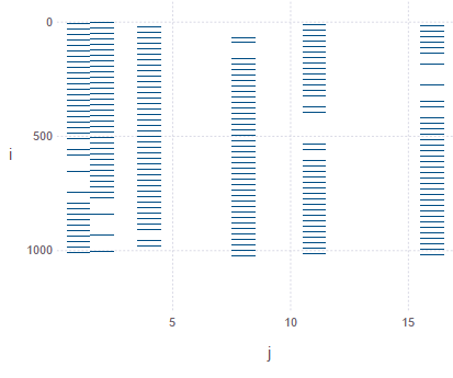
We can already see that the results are all arranged in a small number of columns, and if we zoom into the first 50 rows
spy(qbit[1:50,:])
we start to see the pattern.
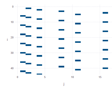
It’s much more clear here that the non-zero values are following a simple repeating pattern. In a perfect world we could just count off the period and use it in further calculations, but since we’re using a quantum computer we can only measure one of those cells, and not all of them. By taking the Fourier transform along the columns however, our qubit will then contain the period(s) of the function.
Here’s where many people (including us) will diverge from the original Shor’s algorithm. While it is feasible to take the quantum Fourier transform of this entire system, it is much faster (and no less accurate) to measure the second register (along the columns). By making this measurement, we will then have only one column of non-zero values, which makes for a much faster Fourier transform.
To simulate making a quantum measurement, we start by finding the square norms of each column
col_norm2 = sum(abs2(qbit),1)
plot(x=collect(1:2^mbits), y = col_norm2, Geom.bar)
And taking a look at it, we see
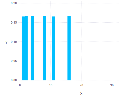
No surprise here, the columns with values have non-zero probabilities, the rest are non-existent. They have (roughly) the same amplitude in each, which means we’re about equally likely to measure any of these columns. We then pick a random number, to get some randomness into our measurement, and compare it to the amplitudes of the columns.
rmeas = rand()
loc=0
for nn=1:2^mbits
     if rmeas < col_norm2[nn]
          loc = nn; break;
     else
          rmeas -= col_norm2[nn]
     end
end
At this point your results and mine will differ, that’s the fun of a random measurement. Don’t worry though, we should still end up with the same results.
Next up we want to take a look at that last column. The first 50 rows look like
plot(x=collect(1:100), y = abs(rem_col[1:100]), Geom.bar)
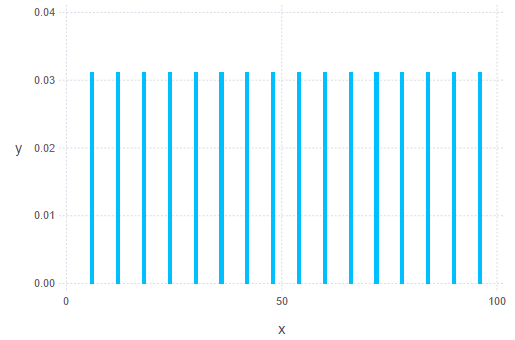
Again, we have a nice evenly distributed set of qubits. Now because we want to find the period of the pattern, we take the Fourier transform, and re-normalize.
rem_fft=fft(qbit[:,loc])
rem_fft./=sum(abs(rem_col))
plot(x=collect([2:2^auxbits]), y = abs(rem_fft[2:2^auxbits]),Geom.bar)
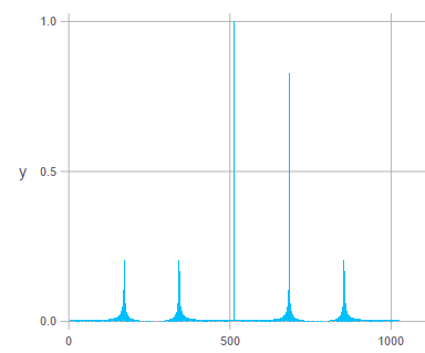
Now we see we have a few large peaks, which we are most likely to measure later on. These are the dominant frequencies in the column we selected, and these are generally integer multiples of the period we’re trying to measure. So we make a quantum measurement on our remaining register, and then we can start working on guessing our period.
loc=0
for nn=1:2^auxbits
  if rmeas < abs(rem_col[nn])
      loc = nn; break;
  else
      rmeas -= abs(rem_col[nn])
  end
end

c = loc-1
Where $c$ is our measurement of the frequency of the pattern. In a perfect world we could simply flip it to find the period, the period would be a perfect integer, and that would be that. However if you look at the plot above, you can see the peaks have some width, so there’s going to be some variance in what we measure.
What we want to do is scan over a set of integer numbers $z$, and find the $z$ for which the value of $\frac{zc}{2^{10}}$ is closest to an integer. I will claim that the $z$ will be somewhere between $m-3\sqrt{m}$ and $m+1-2\sqrt{m}$. So we calculate the lower and upper bounds of this range, then classically iterate over the integers within using:
offset = ceil(m-3*sqrt(m))
diff = floor(m +1 - 2*sqrt(m)) - offset
dist = zeros(convert(Int,diff+1),1)
[dist[nn+1] = abs( (nn+offset)*c/2^auxbits - round((nn+offset)*c/2^auxbits)) for nn=0:diff]
And we can grab the index of the result closest to an integer, and account for the offset to give the value $s$, which is the order of $r$, the result we need to find the prime factors of $m$.
There are a handful of methods to find the powers now, but the simplest conceptually is to find the gcd of s and m.
s = indmin(dist) + offset -1
agcd=gcd(convert(Int,s),m)
s,agcd , m/agcd
(9.0,3,7.0)
And we can see that 3 and 7 are the prime roots of 21.
Now if you’re following along, and didn’t get the same answer, try running the program again. The probabilistic measurements mean that the algorithm is not guaranteed to find the correct answer every time. Sometimes it might take a couple tries to get the right result, but thankfully the results are easy to check for validity.