Imaginary numbers are a powerful mathematical tool, however most people are only really familiar with the commonly used $i=\sqrt{-1}$. This is fair, because $i$ has uses in just about any technical field you can name, but there are others which have their own uses.
The dual numbers work by a definition similar to the complex numbers that $x = a + b\varepsilon$, where $\varepsilon$ is an imaginary number such that $\varepsilon^2=0$, but $\varepsilon \ne 0$
The usefulness of dual numbers appears when you consider the Taylor series expansion for a general function using $a+b\varepsilon$.
$f(a+b\varepsilon)=\sum_{n=0}^\infty \frac{f^{(n)}(a)b^n\varepsilon^n}{n!} = f(a)+bf^{‘}(a)\varepsilon$
Where higher order terms of $\varepsilon$ drop off because $\varepsilon^2 = 0$.
In programming, we can take advantage of this to retrieve both the value of a function and it’s derivative, even in cases where we don’t know the derivative, or even when the function is a black box.
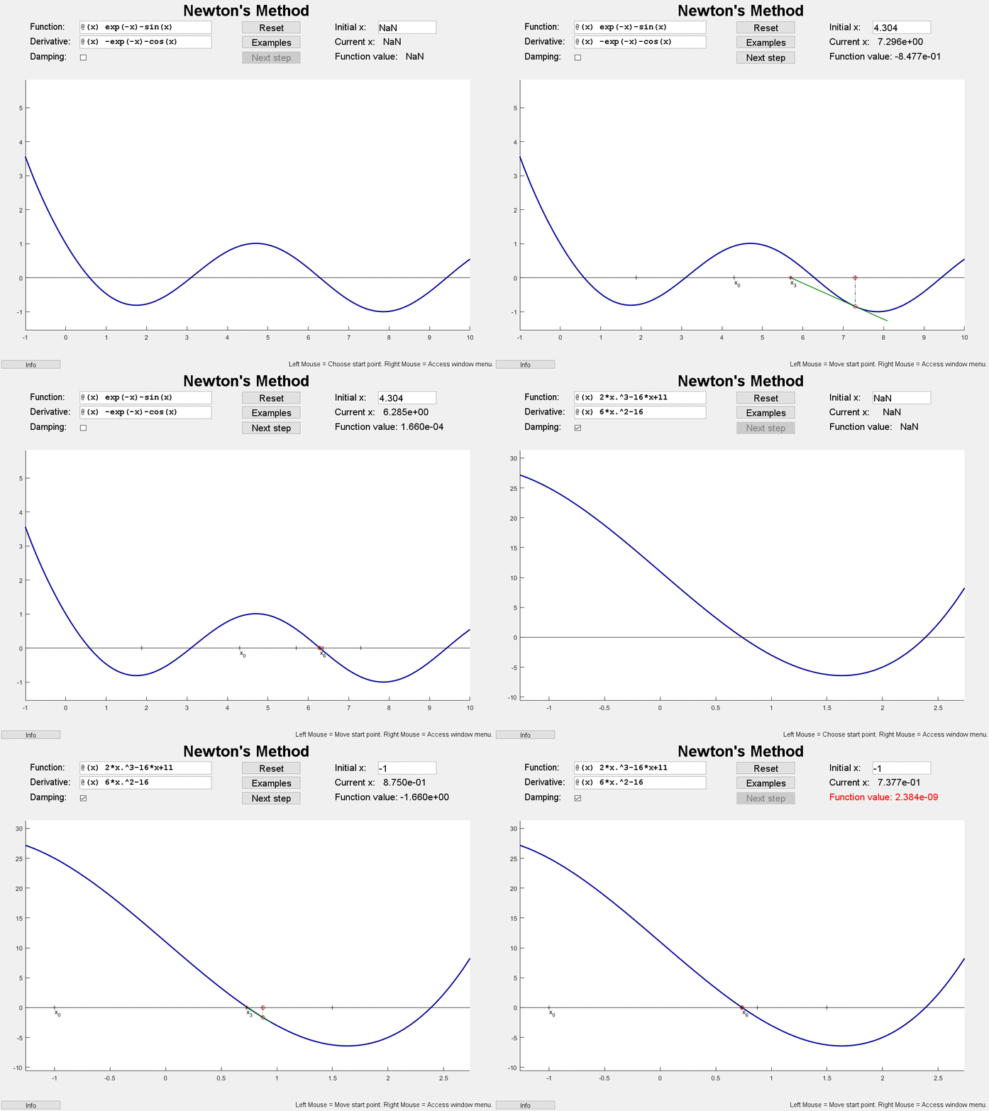
Here’s an example using Julia and the package DualNumbers, but similar packages exist for most common languages. The code below is a simple implementation of Newton’s method for root finding, which is a good use because it allows us to use both the function value and its derivative from each function evaluation. (Note that each function evaluation will require more operations than we would by evaluating with a purely real number. This is because adding and subtracting require 2 operations each, and multiplication and division many more).
We start by defining the function under test in line 3, for this example it’s a simple quadratic, but it certainly doesn’t need to be. Line 4 defines our dual number, this syntax lets us set $x=5+1\varepsilon$. We then evaluate the function at x, and store this in y. The variable y now contains a dual number of the form $y=a+b\varepsilon$, where $a=f(5)$ and $b=\varepsilon\frac{d}{dx}f(5)$.
The actual work of netwons method is in line 10, where we set
$x^{*} = x - \frac{f(x)}{f^{‘}(x)}$ We use
real(y)
to retrieve the value of the function at x, and then
epsilon(y)
to find the derivative. We then find the new value of y, and continue refining x until converges. The results are shown below the code.
using DualNumbers

f(x) = x^2 - 2
x = dual(5,1);
y=f(x)

@printf "\n\n%8s %12s %12s\n" "x" "y" "dy/dx"

while abs(real(y)) > 1e-8
     x = x - real(y)/epsilon(y)
     y = f(x)
     @printf "%8f %8e %8e\n" real(x) real(y) epsilon(y)
end
       x              y          dy/dx
5.000000   2.300000e+01   1.000000e+01
2.700000   5.290000e+00   5.400000e+00
1.720370   9.596742e-01   3.440741e+00
1.441455   7.779358e-02   2.882911e+00
1.414471   7.281571e-04   2.828942e+00
1.414214   6.625248e-08   2.828427e+00
1.414214   4.440892e-16   2.828427e+00
It’s worth noting that things don’t to end here. By implementing your vectors using dual numbers rather than reals, you can easily compute gradients of multidimensional functions, or even the Jacobian of a vector-valued function. If you want to retrieve the second derivative of a function as well (perhaps to implement Halley’s Method), you can use Hyper-Dual numbers, which simply add another different $\varepsilon$, and have an associated Julia Package.
